Quick Demo: Reference-based simulation for Xenium spatial transcriptomics data
[1]:
import simspace as ss
import pandas as pd
[2]:
# Step 1: Load the reference dataset. We here provide a sample dataset from Xenium human breast tumor dataset.
ref_meta = pd.read_csv('../data/reference_metadata.csv', index_col=0)
ref_omics = pd.read_csv('../data/reference_count.csv', index_col=0)
[3]:
ref_meta.head(3)
[3]:
| cell_id | x_centroid | y_centroid | transcript_counts | control_probe_counts | control_codeword_counts | total_counts | cell_area | nucleus_area | Cluster | |
|---|---|---|---|---|---|---|---|---|---|---|
| 0 | 4303 | 1654.367181 | 2017.908301 | 416 | 0 | 0 | 416 | 490.216250 | 82.184375 | Stromal |
| 1 | 4304 | 1669.259509 | 2026.475952 | 560 | 1 | 0 | 561 | 348.741719 | 110.226406 | Invasive_Tumor |
| 2 | 4305 | 1660.068158 | 2040.800818 | 315 | 0 | 0 | 315 | 256.668125 | 65.702344 | Invasive_Tumor |
[4]:
ref_omics.head(3)
[4]:
| 4303 | 4304 | 4305 | 4306 | 4307 | 4308 | 4309 | 4310 | 4311 | 4312 | ... | 76380 | 76381 | 76382 | 76383 | 76384 | 76385 | 76386 | 76387 | 76388 | 76389 | |
|---|---|---|---|---|---|---|---|---|---|---|---|---|---|---|---|---|---|---|---|---|---|
| ABCC11 | 0 | 16 | 4 | 5 | 2 | 0 | 1 | 0 | 0 | 0 | ... | 0 | 1 | 2 | 5 | 3 | 7 | 3 | 1 | 1 | 5 |
| ACTA2 | 13 | 2 | 1 | 0 | 2 | 0 | 1 | 3 | 4 | 13 | ... | 5 | 0 | 0 | 1 | 1 | 0 | 2 | 2 | 0 | 0 |
| ACTG2 | 1 | 1 | 1 | 0 | 2 | 2 | 3 | 6 | 2 | 4 | ... | 1 | 2 | 0 | 4 | 1 | 2 | 3 | 1 | 1 | 4 |
3 rows × 2032 columns
[5]:
# Step 2: Fit SimSpace spatial parameters from the reference.
# This step uses the reference metadata and omics data to fit the spatial parameters for the simulation.
# One can do this by using the `ss.fit()` method and some preprocessing, which is shown in details in spaital_fitting.ipynb.
# Here we provide a pre-fitted parameters for the Xenium human breast tumor dataset, which is fitted
# using the `ss.fit()` method with 100 population size and 40 iterations.
# Note that the 'ss.fit()' method may involve randomness, so the results may vary slightly each time it is run.
params = ss.util.load_params('../data/fitted_params.json')
[6]:
# Step 3: Simulate the spatial omics data using the fitted parameters.
# This step uses the fitted parameters to simulate the spatial omics data, just as the reference-free simulation.
sim = ss.util.sim_from_params(
    parameters=params,
    shape=(100, 100),
    custom_neighbor=ss.spatial.generate_offsets(3, method='manhattan'),
    seed=0,
)
# This results is the simulated spatial omics data shown in Fig. 3, with x and y axis switched.
sim.plot(figsize=(5, 5), dpi=100, size=14)

[6]:
# Step 4 (Optional): Simulate omics data based on the spatial simulation.
# The omics profile can also be fitted from the reference dataset if the reference is available.
# Here we use the `fit_scdesign` method to fit the spatial simulation with the reference dataset,
# which requires the R package 'scDesign3' to be installed. One can find more details in README about the installation.
# The following process may take a while, depending on the size of the reference dataset.
# In this example, it takes about 2 minutes to get the simulation done.
sim.fit_scdesign(
    '../data/reference_count.csv',
    '../data/reference_metadata.csv',
    'Cluster',      # Column in metadata that contains the cell type information
    'x_centroid',   # Column in metadata that contains the x coordinate of the cell centroid
    'y_centroid',   # Column in metadata that contains the y coordinate of the cell centroid
    seed=0,
)
Temporary directory created.
scDesgin fit complete.
[7]:
# Example of plotting a specific gene, e.g., 'CD93'.
sim.plot('CD93', figsize=(5,5), dpi=100)

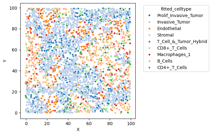
[9]:
sim.plot('fitted_celltype', figsize=(7,7), dpi=100)
[ ]: