Quick Demo: Reference-free spatial omics simulation
[1]:
import numpy as np
import pandas as pd
import matplotlib.pyplot as plt
import seaborn as sns

import simspace as ss
[2]:
# Step 1: Generate random parameters for the simulation. The random parameters will define the characteristics of the spatial omics simulation.
# Here, we generate parameters for 3 groups (niches) and 8 states (cell types), with a fixed seed for reproducibility.
# The parameters include information about the spatial structure, such as the number of groups, states, and other simulation settings.

params = ss.util.generate_random_parameters(
    n_group=3,
    n_state=8,
    seed=42,
)
[ ]:
# Step 2: Create a spatial simulation using the generated parameters.
# The shape of the simulation is set to (100, 100), meaning a 100x100 grid.
# The custom_neighbor argument specifies the spatial connectivity, using Manhattan distance offsets for neighbors.
# One can check the spatial connectivity by sim.neighborhood
# The seed is set to 42 for reproducibility.
sim = ss.util.sim_from_params(
    parameters=params,
    shape=(100, 100),
    custom_neighbor=ss.spatial.generate_offsets(3, method='manhattan'),
    seed=42,
)
[ ]:
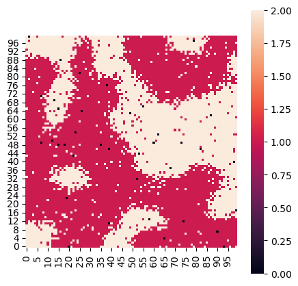
# Step 3: Visualize the spatial simulation.
# The simulation can be visualized using the plot_niche method, which shows the spatial distribution of different niches.
sim.plot_niche(figsize=(5, 5), dpi=100)
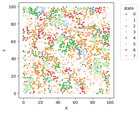
# The plot method can be used to visualize the entire simulation, including the spatial distribution of states.
sim.plot(figsize=(5, 5), dpi=100, size=14)
[ ]:
# Step 4 (Optional): Simulate omics data based on the spatial simulation.
# The create_omics method generates omics data with specified parameters.
# Here, we create 100 genes with a background ratio of 0.6 and a ligand-receptor ratio of 0.2.
# The background and marker parameters define the distribution of gene expression levels.
# The spatial argument is set to False, indicating that the omics data is not spatially dependent.
# The generated omics data can be used for further analysis or visualization.
sim.create_omics(
    n_genes=100,
    bg_ratio=0.6,
    lr_ratio=0.2,
    bg_param = (1, 0.5),
    marker_param = (5, 1.6),
    spatial=False)

sim.gene_meta.head()
| GeneID | Marker | LRindex | Type_0 | Type_1 | Type_2 | Type_3 | Type_4 | Type_5 | Type_6 | Type_7 | |
|---|---|---|---|---|---|---|---|---|---|---|---|
| 0 | 0 | 6 | -1 | 0.026426 | 0.163313 | 1.194430 | 0.136930 | 0.078265 | 0.336136 | 12.154214 | 0.138572 |
| 1 | 1 | -1 | -1 | 0.651374 | 0.229261 | 0.500252 | 0.501919 | 0.383693 | 0.047315 | 0.901822 | 0.193405 |
| 2 | 2 | -1 | -1 | 0.103216 | 0.020815 | 0.446889 | 0.565926 | 0.008363 | 0.358815 | 0.128412 | 0.518062 |
| 3 | 3 | -1 | -1 | 0.095802 | 0.587106 | 0.244479 | 1.380172 | 0.073972 | 0.208566 | 0.060222 | 1.293095 |
| 4 | 4 | 2 | 39 | 1.049167 | 0.149164 | 10.378855 | 0.849742 | 0.405066 | 0.377140 | 0.138439 | 0.048863 |
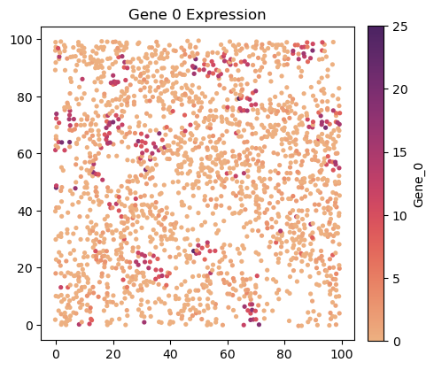
[9]:
ss.plot.plot_gene(
    sim.meta, sim.omics['Gene_0'], size=14,
    figsize=(5,5), dpi=100, title='Gene 0 Expression',
    )